Canterbury Christ Church College

Computing Services - On-line Tutorials

Microsoft Excel Part 3: Opening Files, Highlighting, Inserting Rows and Columns, Formatting cells, Alignment, Fonts, Sizes

OPENING FILES This tutorial assumes that you have already entered and saved the sheet produced in the tutorial Microsoft Excel Part 1 If not you will have to create a spreadsheet similar to the one shown below right	To Open and Existing Spreadsheet file from floppy disk Open Excel Place the Floppy Disk in the diskette drive Double click on the Excel7 icon using the left button of the mouse Click on the File Open icon i.e. 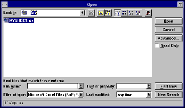You will see Click on the select button and choose the A drive You will see something like: Double Click on your saved file, which should load To open a file saved on the network Repeat the above but choose drive N instead of drive A The opened spreadsheet should display data something similar to
HIGHLIGHTING Before you change the font, size or format of cells your spreadsheet, Excel will need to know which cells you want to change. This is done by Highlighting You can highlight a group of cells, rows, columns or the whole spreadsheet.	To highlight a group of cells Move to any cell Click and hold down the left button of the mouse and drag to another part of the sheet. The area should be highlighted e.g. 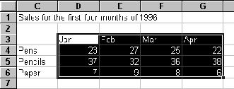To highlight Rows and Columns Move to the Row margin Click on a number. The row should highlight e.g. Click on a column heading to highlight a column Dragging across several row numbers or several column headings will highlight groups of rows or columns To highlight the whole sheet Click on the button at the top of the rows and left of the column headings. e.g. 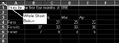To highlight separate areas on a sheet Highlight the first area as indicated above Hold down the key and highlight the second area
INSERTING ROWS AND COLUMNS Excel always inserts arow immediately above the one selected If entering rows into a set of figures on which a calculation is based e.g. Summing Columns, the new row should be inserted somewhere between existing rows. Otherwise the formulae will not be updated	To Insert a row or column into our spreadsheet Move to and click on the margin of row 5. (Whole row should highlight.) From the menu Select Edit, Select Insert (A new row 5 should be inserted) Note the procedure is the same for inserting a column Move to cell B9 (Note how the formula has been updated) Enter the data on folders for the new row 5. Note how the totals automatically update
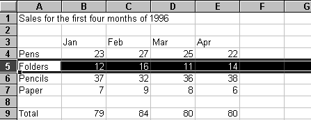
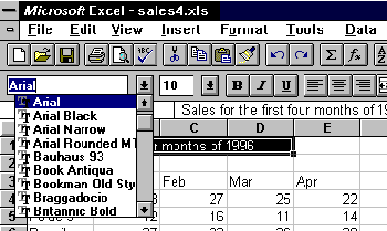
CHANGING FORMATS Excel allows us to change the font, size, style, alignment and format ( e.g. no. of decimal points, type of date) of all cells.	To change fonts and sizes. Example: Move the cursor to cell Al Click and drag the mouse cursor through the text From the ToolBars select the Fonts pull down button Change the Font to ARIAL From the ToolBars select the Size pull down button Change the Size to 14 To change cell alignment. Example: Move to and click on the margin of row 3. (Whole row should highlight.) Select the right align icon . Months of the year should be right-aligned To change cell STYLE (Bold / Underline / Italics). Example: Highlight the whole of row 9 Select the BOLD icon: Experiment similarly with Italic and Underline for other rows and columns To change cell format , Example: Number of Decimal places Move to cell B4. 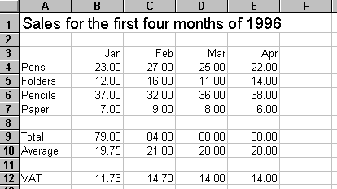Click and drag the mouse down to cell E12. To highlight all the numeric cells from B4 to E12 From the ToolBars select the Increase Decimal Icon Click twice to add two decimal places to your numbers You should see:
SAVING YOUR TUTORIAL If you wish to use your spreadsheet again save your work, following the instructions given in the tutorial Excel Part 1

This tutorial have been created by The TITLE Unit
This tutorial was created on 25th September, 1996
Last Revised: