Canterbury Christ Church College

Computing Services - On-line Tutorials

Microsoft Excel Part 5: Introduction to Charts

CHARTS The easiest way to produce charts in Excel is by using the Chart Wizards. The full Chart Wizard icon appears on the Standard ToolBar. Selecting this icon takes you through a series of very simple screens in which you create a graph of your choice from the area you have highlighted. The Default Column Chart Wizard icon (On the Chart ToolBar) creates a column chart directly from your highlighted area	To Create a Simple Column Chart using the Chart Wizard. 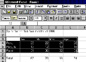Example: Either load the file saved at the end of Excel lesson 1 or create a spreadsheet similar to the one below. Move to cell A3. Click and drag the mouse down to cell E7. (All the cells A3 to E6 should be highlighted.) From the TOOL BAR Select Chart Wizard (A Dotted Line should now be circulating around the block A3 to E7) Move to cell B13. Place the cursor (now a black cross) on the top left comer of the cell. Click and drag the mouse down to cell G26 this creates an area to place the chart. 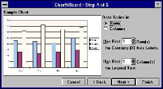A series of Chart Wizard prompt screens will appear: Chart Wizard STEP 1 Select Next Chart Wizard STEP 2 Select Column, Select Next Chart Wizard STEP 3 Select 1, Select Next Chart Wizard STEP 4 Select Next Chart Wizard STEP 5 Chart Title : Enter SALES Y axis : Enter PROFIT Select OK A bar chart with legends based on the above figures should appear in the area B13-G26
DEFAULT COLUMN CHARTS The Default Column Chart icon appears on the Chart ToolBar which does not automatically appear on loading Excel. The Chart and other ToolBars can be switched on and off using the View Menu	To Create a Simple Column Chart using the Default Column Chart Wizard. Example Move to cell A3. Click and drag the mouse down to cell E7. (All the cells A3 to E6 should be highlighted.) From the Menu select View, select ToolBars, select Chart You should see From the Chart ToolBar Select Default Column Chart Wizard (A Dotted Line should now be circulating around the block A3 to E7) Move to cell B13. Place the cursor (now a black cross) on the top left comer of the cell. Click and drag the mouse down to cell G26 this creates an area to place the chart. A bar chart with legends based on the above figures should appear in the area B13-G26
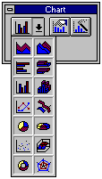
MODIFYING CHARTS It is very easy to change your column chart to some other form e.g. Line Graph, Bar Chart, Pie Chart, etc. Charts can also be displayed in 3D format. The example opposite gives one example of such a change Later tutorials will deal with changing axes, titles, colours, labels, alignment, etc.	To change a chart to another format On the Chart Toolbar select the Chart Type Pulldown Select the 3D pie chart Experiment with other chart displays by selecting from the Chart Tool Bar. The difficulty is not in creating charts - but to be able to select the right type to display the information you have - it is easy to get carried away!!
SAVING YOUR TUTORIAL	To save your work From the ToolBar select the SAVE icon To save it to a floppy disk type A and a colon in front of your filename e.g. A:FILENAME (Filenames should be 8 characters or less with no spaces) Press Enter If presented with a Summary Frame you may enter details or just press Enter To save the file to your area on the network, repeat the above but omit the A: in front of FILENAME.

This tutorial have been created by The TITLE Unit
This tutorial was created on 25th September, 1996
Last Revised: